Trajectory3D
class phaseportrait.Trajectory3D(dF, *, Range=None, dF_args={}, n_points=10000, runge_kutta_step=0.01, runge_kutta_freq=1, **kargs)
Inherits from parent class trajectory.
Gives the option to represent 3D trajectories given a dF function with 3 args.
Parameters
-
dF : callable
A dF type function.
Key Arguments
-
Range : list
Ranges of the axis in the main plot, by default None. See Defining Range.
-
dF_args : dict
If necesary, must contain the kargs for the
dFfunction, by default {} -
n_points : int
Maximum number of points to be calculated and represented, by default 10000
-
runge_kutta_step : float
Step of 'time' in the Runge-Kutta method, by default 0.01
-
runge_kutta_freq : int
Number of times
dFis aplied between positions saved, by default 1 -
xlabel : str
x label of the plot, by default 'X'
-
ylabel : str
y label of the plot, by default 'Y'
-
zlabel : str
z label of the plot, by default 'Z'
Methods
Inherits methods from parent class trajectory, a brief resume is offered, click on the method to see more information:
-
Adds thermalization steps and random initial position.
-
Adds a trajectory with the given initial position.
-
Adds multiple trajectories with the given initial positions.
-
plot :
Prepares the plots and computes the values. Returns the axis and the figure.
-
Adds a slider for the dF function.
Defining Range
-
A single number. In this case the range is defined from zero to the given number in all axes.
-
A range, such
[lowerLimit , upperLimit]. All axes will take the same limits. -
Three ranges, such that
[[xAxisLowerLimit , xAxisUpperLimit], [yAxisLowerLimit , yAxisUpperLimit], [zAxisLowerLimit , zAxisUpperLimit]]
Examples
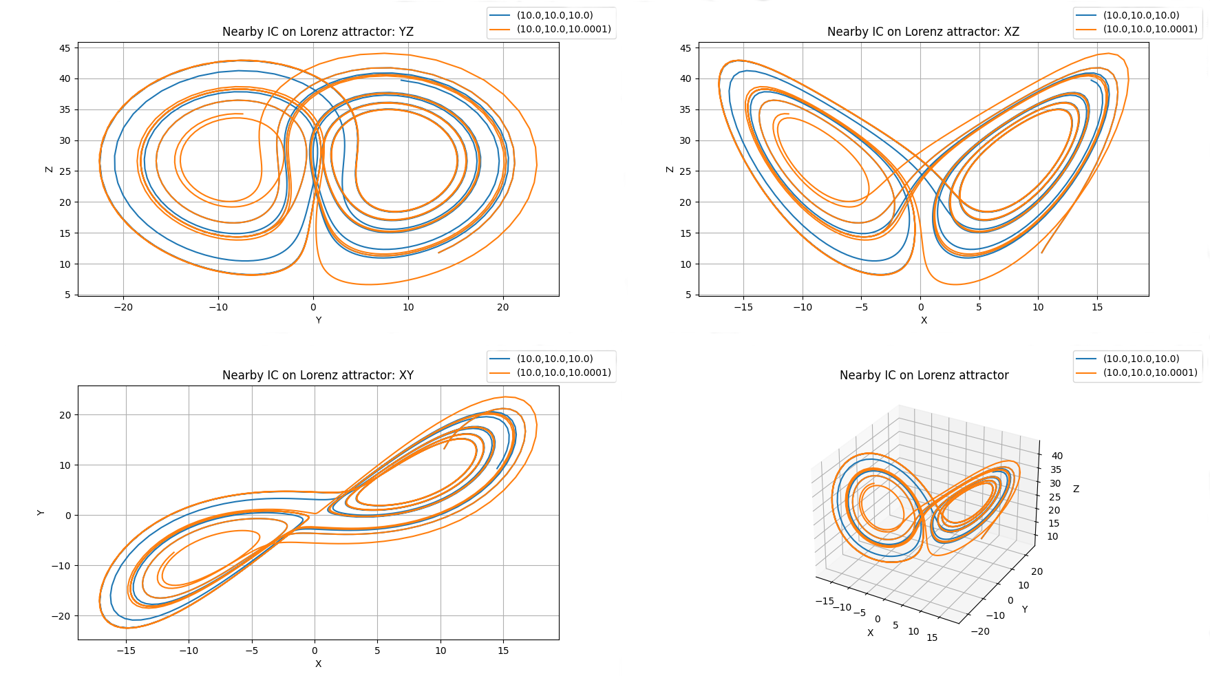
Lorentz attractor: chaos
Two trajectories with similar initial positions under the influence of Lorentz equations.
from phaseportrait import Trajectories3D

def Lorenz(x,y,z,*, s=10, r=28, b=8/3):
    return  -s*x+s*y,
            -x*z+r*x-y,
            x*y-b*z

a = Trajectory3D(
    Lorenz,
    lines=True,
    n_points=1300,
    size=3,
    mark_start_position=True,
    Title='Nearby IC on Lorenz attractor'
    )

a.initial_position(10,10,10)
a.initial_position(10,10,10.0001)
a.plot()
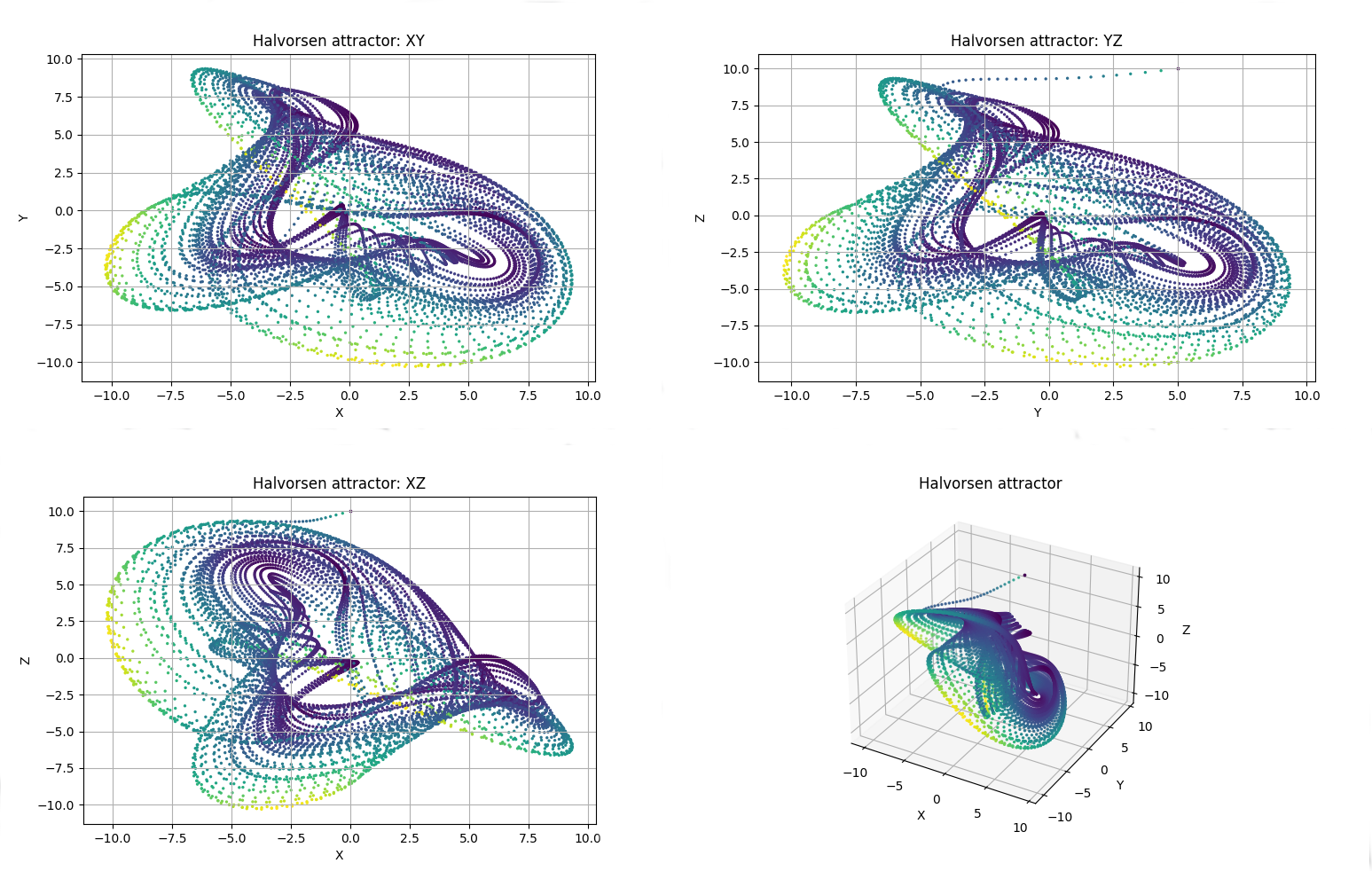
Halvorsen attractor
In this example we are interested in seeing the attractor, not trajectories, under the Halvorsen equations.
from phaseportrait import Trajectories3D

def Halvorsen(x,y,z, *, s=1.4):
    delta = (3*s+15)
    return  -s*x+2*y-4*z-y**2+delta,
            -s*y+2*z-4*x-z**2+delta,
            -s*z+2*x-4*y-x**2+delta

d = Trajectory3D(
    Halvorsen,
    dF_args={'s':1.4},
    n_points=10000,
    thermalization=0,
    numba=True,
    size=2,
    mark_start_point=True,
    Title='Halvorsen attractor'
    )

d.initial_position(0,5,10)
d.plot()